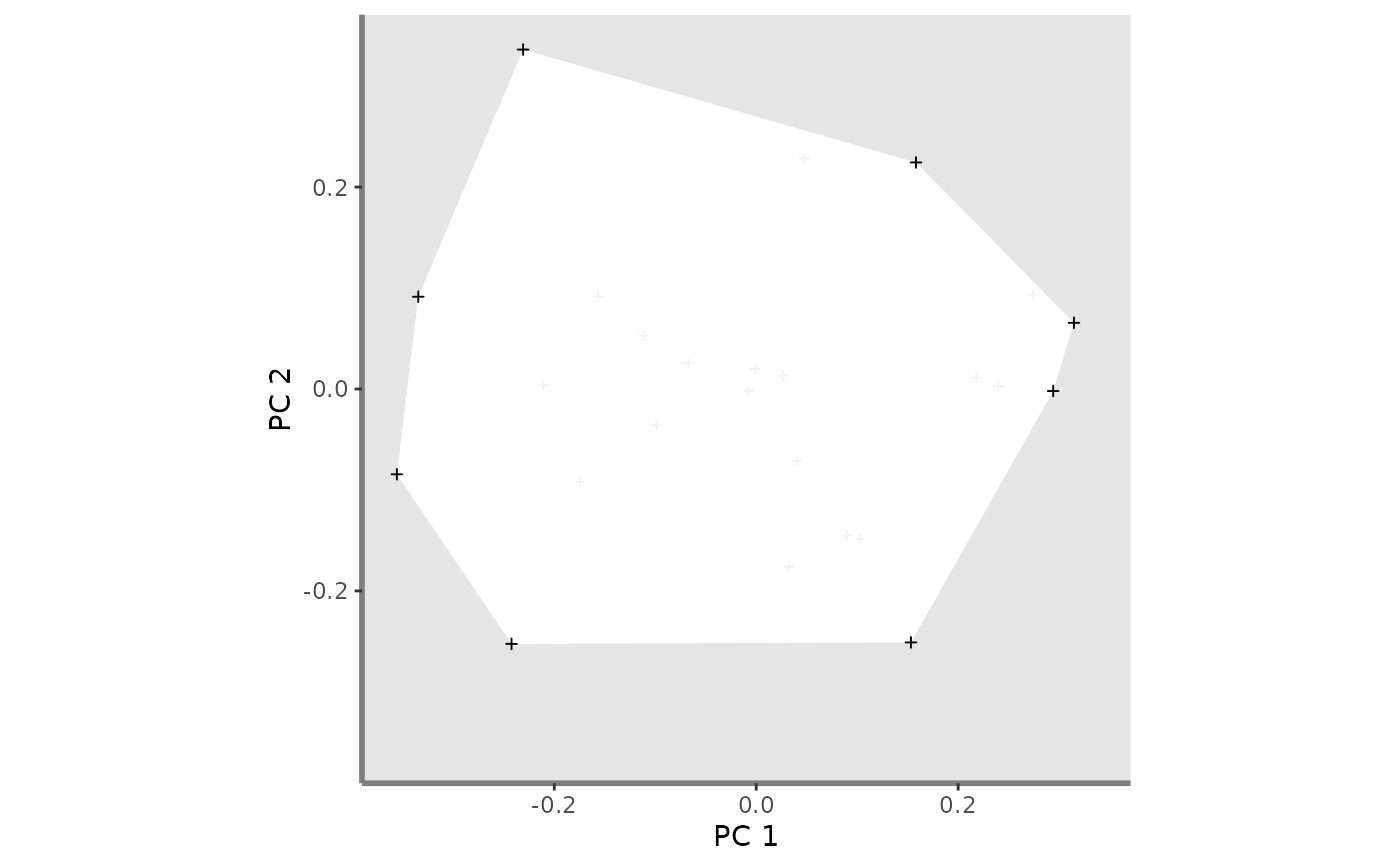
Plot species from the pool — pool.plot • mFD

Plot all species from the study case and associated convex hull

pool.plot(
  ggplot_bg,
  sp_coord2D,
  vertices_nD,
  plot_pool = TRUE,
  shape_pool = 3,
  size_pool = 0.8,
  color_pool = "grey95",
  fill_pool = NA,
  color_ch = NA,
  fill_ch = "white",
  alpha_ch = 1,
  shape_vert = 3,
  size_vert = 1,
  color_vert = "black",
  fill_vert = NA
)

Arguments

ggplot_bg: a ggplot object of the plot background retrieved through the background.plot function.
sp_coord2D: a list of matrix (ncol = 2) with coordinates of species present in the pool for a given pair of axes
vertices_nD: a list (with names as in sp_coord2D) of vectors with names of species being vertices in n dimensions.
plot_pool: a logical value indicating whether species of each assemblage should be plotted or not. Default: plot_pool = TRUE.
shape_pool: a numeric value referring to the shape used to plot species pool. Default: shape_pool = 16(filled circle).
size_pool: a numeric value referring to the size of species belonging to the global pool. Default: size_pool = 1.
color_pool: a R color name or an hexadecimal code referring to the color of the pool. This color is also used for FRic convex hull color. Default: color_pool = "#0072B2".
fill_pool: a R color name or an hexadecimal code referring to the colour to fill species symbol (if shape_sp > 20) and the assemblage convex hull. Default: fill_pool = '#0072B2'.
color_ch: a R color name or an hexadecimal code referring to the border of the convex hull filled by the pool of species. Default: color_ch = "black".
fill_ch: a R color name or an hexadecimal code referring to the filling of the convex hull filled by the pool of species. Default is: fill_ch = "white".
alpha_ch: a numeric value for transparency of the filling of the convex hull (0 = high transparency, 1 = no transparency). Default: alpha_ch = 0.3.
shape_vert: a numeric value referring to the shape used to plot vertices if vertices should be plotted in a different way than other species. If shape_vert = NA, no vertices plotted. Default: shape_vert = NA.
size_vert: a numeric value referring to the size of symbol for vertices. Default: size_vert = 1.
color_vert: a R color name or an hexadecimal code referring to the color of vertices if plotted. If color_vert = NA, vertices are not plotted (for shapes only defined by color, ie shape inferior to 20. Otherwise fill must also be set to NA). Default: color_vert = NA.
fill_vert: a character value referring to the color for filling symbol for vertices (if shape_vert >20). If fill = NA and color = NA, vertices are not plotted (if shape_vert superior to 20. Otherwise color_vert = NULL is enough). Default is NA.

Value

A ggplot object plotting background of multidimensional graphs and species from the global pool (associated convex hull if asked).

Author

Camille Magneville and Sebastien Villeger

Examples

# Load Species*Traits dataframe:
data("fruits_traits", package = "mFD")

# Load Assemblages*Species dataframe:      
data("baskets_fruits_weights", package = "mFD") 

# Load Traits categories dataframe:
data("fruits_traits_cat", package = "mFD") 
 
# Compute functional distance 
sp_dist_fruits <- mFD::funct.dist(sp_tr         = fruits_traits,
                                  tr_cat        = fruits_traits_cat,
                                  metric        = "gower",
                                  scale_euclid  = "scale_center",
                                  ordinal_var   = "classic",
                                  weight_type   = "equal",
                                  stop_if_NA    = TRUE)
#> [1] "Running w.type=equal on groups=c(Size)"
#> [1] "Running w.type=equal on groups=c(Plant)"
#> [1] "Running w.type=equal on groups=c(Climate)"
#> [1] "Running w.type=equal on groups=c(Seed)"
#> [1] "Running w.type=equal on groups=c(Sugar)"
#> [1] "Running w.type=equal on groups=c(Use,Use,Use)"
  
# Compute functional spaces quality to retrieve species coordinates matrix:
fspaces_quality_fruits <- mFD::quality.fspaces(sp_dist = sp_dist_fruits, 
 maxdim_pcoa         = 10,
 deviation_weighting = "absolute",
 fdist_scaling       = FALSE,
 fdendro             = "average")
 
# Retrieve species coordinates matrix:
sp_faxes_coord_fruits_2D <- 
  fspaces_quality_fruits$details_fspaces$sp_pc_coord[ , c("PC1", "PC2")]

# Set faxes limits:
# set range of axes if c(NA, NA):
 range_sp_coord_fruits  <- range(sp_faxes_coord_fruits_2D)
 range_faxes_lim <- range_sp_coord_fruits + 
   c(-1, 1)*(range_sp_coord_fruits[2] - 
   range_sp_coord_fruits[1]) * 0.05
 
 # Retrieve the background plot:
 ggplot_bg_fruits <- mFD::background.plot(
                               range_faxes = range_faxes_lim, 
                               faxes_nm    = c("PC 1", "PC 2"), 
                               color_bg    = "grey90") 
                               
 # Retrieve vertices names:
 vert_nm_fruits <- vertices(sp_faxes_coord_fruits_2D, 
  order_2D = TRUE, check_input = TRUE)
  
 # Plot the pool:
 plot_pool_fruits <- pool.plot(ggplot_bg   = ggplot_bg_fruits,
           sp_coord2D    = sp_faxes_coord_fruits_2D,
           vertices_nD   = vert_nm_fruits,
           plot_pool     = TRUE,
           shape_pool    = 3, 
           size_pool     = 0.8, 
           color_pool    = "grey95", 
           fill_pool     = NA, 
           color_ch      = NA, 
           fill_ch       = "white", 
           alpha_ch      = 1, 
           shape_vert    = 3, 
           size_vert     = 1, 
           color_vert    = "black", 
           fill_vert     = NA) 
 plot_pool_fruits